library(duckdb)
library(DBI)

con <- DBI::dbConnect(
  duckdb::duckdb(),
  "data/GiBleed_5.3_1.1.duckdb"
)1 Database Concepts
1.1 What is a Database?
A database is an organized collection of structured information, or data, typically stored electronically in a computer system. A database is usually controlled by a database management system (DBMS). Together, the data and the DBMS, along with the applications that are associated with them, are referred to as a database system, often shortened to just database. - Oracle Documentation
When we talk about databases, we often mean the database system rather than database itself. Specifically, we talk about the different layers of a database system.
1.2 Parts of a Database System
The Composable Codex talks about three layers of a database system:
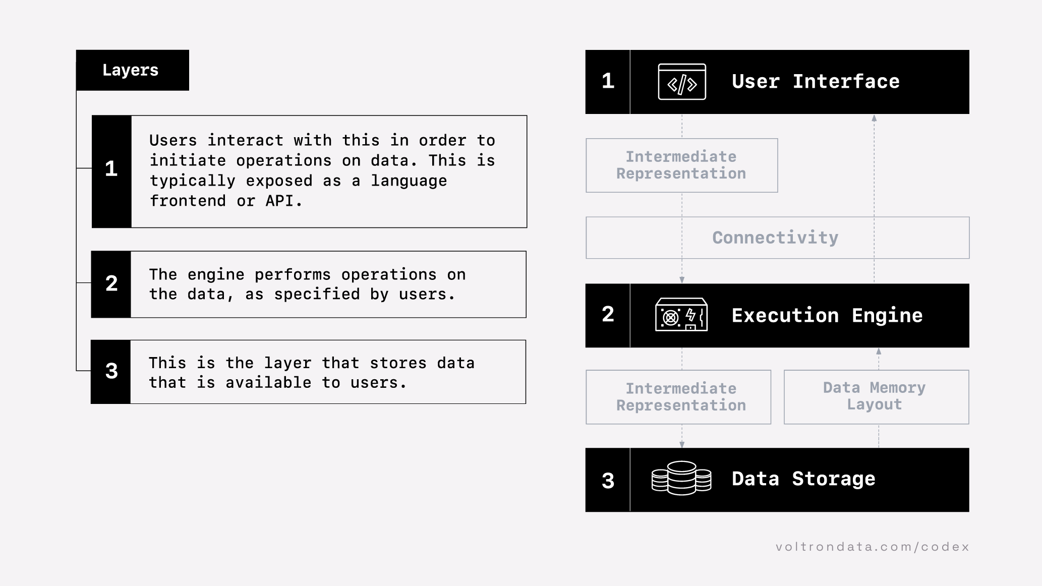
- A user interface - how users interact with the database. In this class, our main way of interacting with databases is SQL (Structured Query Language).
- An execution engine - a software system that queries the data in storage. There are many examples of this: SQL Server, MariaDB, DuckDB, Snowflake. These can live on our machine, on a server within our network, or a server on the cloud.
- Data Storage - the physical location where the data is stored. This could be on your computer, on the network, or in the cloud (such as an Amazon S3 bucket)
1.3 For this class
In our class, we will use the following configuration:
graph TD
A["1.SQL"] --> B
B["2.DuckDB"] --> C
C["3.File on our Machine"]
But you can think of other configurations that might be more applicable to you. For example, a lot of groups at the Hutch use SQL Server:
graph TD
A["1.SQL"] --> B
B["2.SQL Server"] --> C
C["3.FH Shared Storage"]
In many ways, SQL Server and its storage are tightly coupled (the engine and the storage are in the same location). This coupling can make it difficult to migrate out of such systems.
Or, for those who want to use cloud-based systems, we can have this configuration:
graph TD
A["1.SQL/Notebooks"] --> B
B["2.Databricks/Snowflake"] --> C
C["3.Amazon S3"]
In this case, we need to sign into the Databricks system, which is a set of systems that lives in the cloud. We actually will use SQL within their notebooks to write our queries. Databricks will then use the Snowflake engine to query the data that is stored in cloud storage (an S3 bucket).
If this is making you dizzy, don’t worry too much about it. Just know that we can switch out the different layers based on our needs.
1.4 Our underlying data model
The three components of our Database System is dependent on our choice of the data model. Most data models are centered around Relational Databases. A relational database organizes data into multiple tables. Each table’s row is a record with a unique ID called the key, as well as attributes described in the columns. The tables may relate to each other based on columns with the same values.
Below is an example entity-relationship diagram that summarizes relationships between tables:
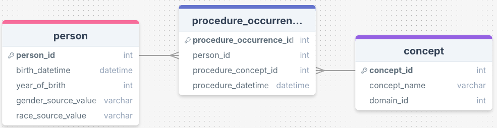
Each rectangle represent a table, and within each table are the columns (fields). The connecting lines shows that there are shared values between tables in those columns, which helps one navigate between tables. Don’t worry if this feels foreign to you right now - we will unpack these diagrams throughout the course.
Other data models include NoSQL (“Not Only SQL”), which allows the organization of unstructured data via key-value pairs, graphs, and encoding entire documents. Another emerging data model are Array/Matrix/Vector-based models, which are largely focused on organizing numerical data for machine learning purposes.
1.5 What is SQL?
SQL is short for Structured Query Language. It is a standardized language for querying relational databases.
SQL lets us do various operations on data. It contains various clauses which let us manipulate data:
| Priority | Clause | Purpose |
|---|---|---|
| 1 | FROM |
Choose tables to query and specify how to JOIN them together |
| 2 | WHERE |
Filter tables based on criteria |
| 3 | GROUP BY |
Aggregates the Data |
| 4 | HAVING |
Filters Aggregated Data |
| 5 | SELECT |
Selects columns in table and calculate new columns |
| 6 | ORDER BY |
Sorts by a database field |
| 7 | LIMIT |
Limits the number of records returned |
We do not use all of these clauses when we write a SQL Query. We only use the ones we need to get the data we need out.
Oftentimes, we really only want a summary out of the database. We would probably use the following clauses:
| Priority | Clause | Purpose |
|---|---|---|
| 1 | FROM |
Choose tables to query and specify how to JOIN them together |
| 2 | WHERE |
Filter tables based on criteria |
| 3 | GROUP BY |
Aggregates the Data |
| 5 | SELECT |
Selects columns in table and calculate new columns |
Notice that there is a Priority column in these tables. This is important, because parts of queries are evaluated in this order.
NoteDialects of SQL
You may have heard that the SQL used in SQL Server is different than other databases. In truth, there are multiple dialects of SQL, based on the engine.
However, we’re focusing on the 95% of SQL that is common to all systems. Most of the time, the SQL we’re showing you in this course will get you to where you want to go.
1.6 Anatomy of a SQL Statement
Let’s look at a typical SQL statement:
SELECT person_id, gender_source_value   # Choose Columns
  FROM person                           # Choose the person table
  WHERE year_of_birth < 2000;            # Filter the data using a criterion
We can read this as:
SELECT the person_id and gender_source_value columns
FROM the person table
ONLY Those with year of birth less than 2000
As you can see, SQL can be read. We will gradually introduce clauses and different database operations.
Note
As a convention, we will capitalize SQL clauses (such as SELECT), and use lowercase for everything else.
1.7 Database Connections
We haven’t really talked about how we connect to the database engine.
In order to connect to the database engine and create a database connection, we may have to authenticate with an ID/password combo or use other methods of authentication to prove who we are.
Once we are authenticated, we now have a connection. This is basically our conduit to the database engine. We can send queries through it, and the database engine will run these queries, and return a result.
graph LR
  A["Our Computer"] --query--> B[Database Engine]
  B --results--> A
As long as the connection is open, we can continue to send queries and receive results.
It is best practice to explicitly disconnect from the database. Once we have disconnected, we no longer have access to the database.
graph LR
  A["Our Computer"] --X--> B[Database Engine]
  B --X--> A
1.8 How is the Data Stored?
Typically, the data in databases is stored in tables, such as the one below:
| person_id | gender_concept_id | year_of_birth | month_of_birth | day_of_birth | birth_datetime | race_concept_id | ethnicity_concept_id | location_id | provider_id | care_site_id | person_source_value | gender_source_value | gender_source_concept_id | race_source_value | race_source_concept_id | ethnicity_source_value | ethnicity_source_concept_id |
|---|---|---|---|---|---|---|---|---|---|---|---|---|---|---|---|---|---|
| 6 | 8532 | 1963 | 12 | 31 | 1963-12-31 | 8516 | 0 | NA | NA | NA | 001f4a87-70d0-435c-a4b9-1425f6928d33 | F | 0 | black | 0 | west_indian | 0 |
| 123 | 8507 | 1950 | 4 | 12 | 1950-04-12 | 8527 | 0 | NA | NA | NA | 052d9254-80e8-428f-b8b6-69518b0ef3f3 | M | 0 | white | 0 | italian | 0 |
| 129 | 8507 | 1974 | 10 | 7 | 1974-10-07 | 8527 | 0 | NA | NA | NA | 054d32d5-904f-4df4-846b-8c08d165b4e9 | M | 0 | white | 0 | polish | 0 |
| 16 | 8532 | 1971 | 10 | 13 | 1971-10-13 | 8527 | 0 | NA | NA | NA | 00444703-f2c9-45c9-a247-f6317a43a929 | F | 0 | white | 0 | american | 0 |
| 65 | 8532 | 1967 | 3 | 31 | 1967-03-31 | 8516 | 0 | NA | NA | NA | 02a3dad9-f9d5-42fb-8074-c16d45b4f5c8 | F | 0 | black | 0 | dominican | 0 |
| 74 | 8532 | 1972 | 1 | 5 | 1972-01-05 | 8527 | 0 | NA | NA | NA | 02fbf1be-29b7-4da8-8bbd-14c7433f843f | F | 0 | white | 0 | english | 0 |
| 42 | 8532 | 1909 | 11 | 2 | 1909-11-02 | 8527 | 0 | NA | NA | NA | 0177d2e0-98f5-4f3d-bcfd-497b7a07b3f8 | F | 0 | white | 0 | irish | 0 |
| 187 | 8507 | 1945 | 7 | 23 | 1945-07-23 | 8527 | 0 | NA | NA | NA | 07a1e14d-73ed-4d3a-9a39-d729745773fa | M | 0 | white | 0 | irish | 0 |
| 18 | 8532 | 1965 | 11 | 17 | 1965-11-17 | 8527 | 0 | NA | NA | NA | 0084b0fe-e30f-4930-b6d1-5e1eff4b7dea | F | 0 | white | 0 | english | 0 |
| 111 | 8532 | 1975 | 5 | 2 | 1975-05-02 | 8527 | 0 | NA | NA | NA | 0478d6b3-bdb3-4574-9b93-cf448d725b84 | F | 0 | white | 0 | english | 0 |
Some quick terminology:
- Database Record - a row in this table. In this case, each row in the table above corresponds to a single person.
- Database Field - the columns in this table. In our case, each column corresponds to a single measurement, such as
birth_datetime. Each column has a specific datatype, which may be integers, decimals, dates, a short text field, or longer text fields. Think of them like the different pieces of information requested in a form.
It is faster and requires less memory if we do not use a single large table, but decompose the data up into multiple tables. These tables are stored in a number of different formats:
- Comma Separated Value (CSV)
- A Single File (SQL Server)
- a virtual file
In a virtual file, the data acts like it is stored in a single file, but is actually many different files underneath that can be on your machine, on the network, or on the cloud. The virtual file lets us interact with this large mass of data as if it is a single file.
The database engine is responsible for scanning the data, either row by row, or column by column. The engines are made to be very fast in this scanning to return relevant records.